I. INTRODUCTION
In the field of computer vision and image processing, neural networks improve their performance noticeably. Image reconstruction restores an original image by referring to given information such as reference pixels. Image reconstruction can be applied to various fields such as intra prediction for video coding, inpainting, and super-resolution. Video coding standards such as AVC [1], HEVC [2], and VVC [3] provide intra modes to reconstruct the image spatially. joint photographic experts group (JPEG) has been promoting the establishment of JPEG-AI, a new image coding standard through artificial intelligence including picture prediction since 2019 [4].
Studies for image reconstruction have been conducted as follows. Convolutional Neural Networks (CNNs) are utilized to obtain local features and to convert feature domain to pixel domain for reconstructing the image. Palmprint reconstruction attack methods [5-7] reconstruct the images to modify the given template images through CNN layers. CNN-based Methods [8-11] reconstruct each pixel of an image by extracting features for a local region. However, these methods have a problem that the same weights are given to the reference pixels although some pixels have low correlation. Sequential pixels in a certain direction can be handled through recurrent neural network (RNN) and Long Short-Term Memory (LSTM) [12] that process arbitrary sequences of inputs. RNN-based methods [13-14] predict a pixel through previous consecutive pixels in a vertical or horizontal direction. However, these networks cause gradient vanishing and exploding in training due to their recursive structure [15]. Therefore, RNN has a long term dependency problem that correlation information is forgotten between two elements whose distance are far. Attention mechanism [16] can solve this problem. Attention mechanism is originally used in natural language processing (NLP) for finding the correlation between tokens embedding each word. Attention mechanism is also applied to computer vision [17-19]. Methods based on attention mechanism has similar or superior performance to the CNN-based methods. Masked autoencoder (MAE) [20] proposes a training method for a ViT-based network by masking some random patches and restructuring them in order to improve the performance.
In this paper, we propose a block reconstruction method by extracting the spatial features of reference pixels and predicting the spatial features of a target block. Vertical and horizontal spatial features are extracted through CNN layers from top and left adjacent blocks, respectively. Atten-tion layers predict the spatial features of a target block by finding a correlation between the target block and the reference pixels. Finally, the pixels of the target block are reconstructed by converting spatial feature domain to pixel domain through CNN layers.
II. RELATED WORKS
RNN has a recursive structure to process sequential data. The output of an RNN cell is back to itself so it is called a 'hidden state'. The hidden state preserves the features of previous inputs. RNN processes the inputs through the hidden state in a certain step. The types of RNNs are vanilla RNN, LSTM [12], and Gated Recurrent Unit (GRU) [21]. The structure of vanilla RNN is simple, but it has the problem of long-term dependency that means losing the features of old inputs. LSTM introduces long-term and short-term states in order to prevent the long-term dependency problem. The short-term state is similar to the hidden state in vanilla RNN. The long-term state forgets a part of itself and adds a part of the short-term state in each step. The features of the old inputs can be preserved through the long-term state. GRU is the simplified structure of LSTM. In GRU, the short-term and long-term states in LSTM are integrated into one hidden state. In GRU, a part of the hidden state is forgotten or added in each step.
Pixels in an image can be regarded as time-series data. Therefore, spatial features can be extracted from pixels in a vertical or horizontal direction through RNN. Y. Hu et al. [13] propose an intra prediction method through RNN layers with various input sizes. The region of reference pixels is scaled to the input sizes. PS-RNN [14] predicts the visual features of the reference pixels through CNN layers. The spatial features are extracted through RNN layers guided by visual features. The pixels of the block are predicted by converting the spatial features to pixel domain. However, training the RNN-based network known to be difficult due to a gradient vanishing or exploding caused by its recursive structure [15].
CNN is also utilized to extract the spatial features. CNN kernels for extracting the spatial features is not square shaped but its height or width is equal to the inputs. The kernels can extract the spatial features in the vertical or horizontal direction. Lee and Kwon [22] extract the spatial features of top and left blocks through CNN layers in order to predict the clusters of pixels in a block. Li et al. [23] find the spatial features for an electrical impedance tomography to reconstruct its 3D shape.
Attention mechanism [16] can selectively focus on the various elements of the inputs, giving more importance to some elements. Attention has three inputs: query, key, and value. The query is an input feature. The key and value are pairs of features corresponding to the query and actual value, respectively. The value is weighted according to similarities between the query and key. Self-attention, whose inputs are the same, is utilized to predict correlations between each element in the input data itself.
Attention mechanism can be applied not only to natural language processing (NLP) but also to image processing. CNN is specialized in extracting image features in local areas, so it has a disadvantage that it is difficult to detect a correlation between two distant pixels. On the other hand, attention can find the correlations for all inputs, so the correlation between two distant pixels can be better detected. Vision Transformation (ViT) [17] classifies an object in an image through encoder networks composed of attention layers. The input image is divided into multiple blocks. The image features are updated by sequentially inputting the blocks into the encoder network. The pixels are regarded as embedded words in NLP. Video Transformer Network (VTN) [18] extracts the spatial features of a video through ViT and detects temporal features through a temporal attention-based encoder. Attention mechanism can better extract global image features than CNN. However, attention mechanism requires a large amount of data for a network training.
III. IMAGE RECONSTRUCTION METHOD BY SPATIAL FEATURE PREDICTION
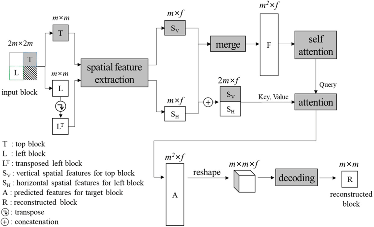
We propose a block reconstruction method by referring adjacent blocks through CNN and attention layers. For a m×m target block in an image, top and left adjacent blocks of the same size are designated as reference pixels. The reference pixels are utilized to obtain vertical and horizontal spatial features, respectively, through CNN layers. Attention mechanism is applied to predict spatial correlations between the target block and the reference pixels. The pixels of the target block are reconstructed through the spatial correlations. Fig. 1 shows the flow of the proposed method.
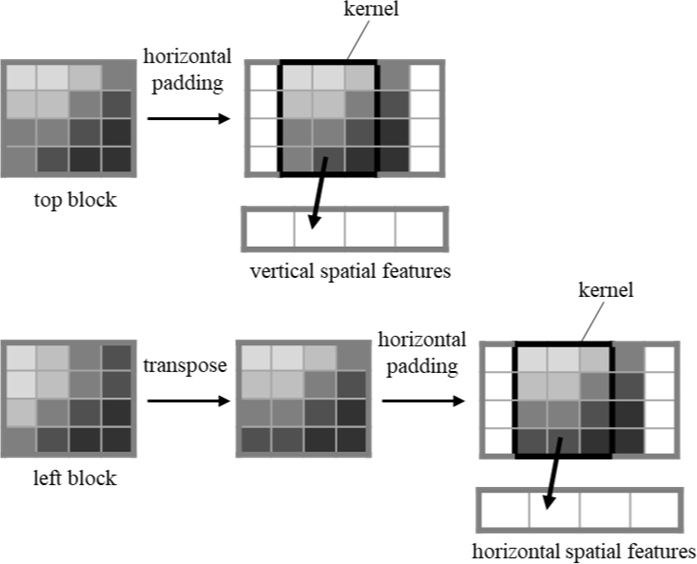
The spatial feature maps for the top and left block are extracted for predicting the spatial features of the target block. For the top and left block, CNN layers extract f local spatial features. Then, vertical spatial features are obtained through a CNN layer with a size of m×3 and that is applying only a horizontal padding. Fig. 2 illustrates the structure of the extraction module for extracting the spatial features.
The module can extract the vertical spatial feature map for the top block. The same module can be utilized to extract horizontal spatial features by transposing the left block before inputting it to the extracting module. This reduces the number of the network weights and improves a network learning efficiency. Fig. 3 shows the spatial feature extraction for the top and left blocks.
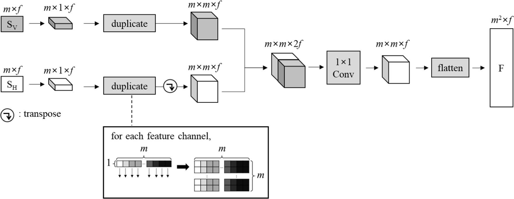
The two spatial feature maps are merged for applying attention mechanism. A dimension for a vertical direction is added into both the two m×f spatial feature maps, then the dimensions of these become m×1×f. The values of the spatial feature maps are duplicated m times in the vertical direction. The spatial feature map for the left block is transposed to have the same value for the same row. The two spatial feature maps are concatenated along the feature dimension. Then, the dimensions are merged for vertical and horizontal directions. Merging the spatial feature maps is represented as follows:
where F is the m2×f matrix for the merged spatial features, SV and SH are the spatial feature maps of the top and left blocks, respectively, i and j are spatial coordinates, respectively, and k is the index of the feature dimension. Fig. 4 shows the flow of merging the spatial feature maps.
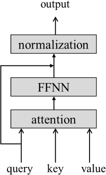
An attention module for detecting the correlations about the inputs consists of an attention, a feed-forward neural network (FFNN), and a normalization as shown in Fig. 5. The attention module has three inputs for the query, key, and value. The first and second dimensions of the input refer to the lengths of element and feature, respectively. The input sizes of the key are equal to the value. The feature lengths of the attention inputs are the same. The output size of the attention module is equal to the input.
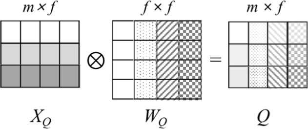
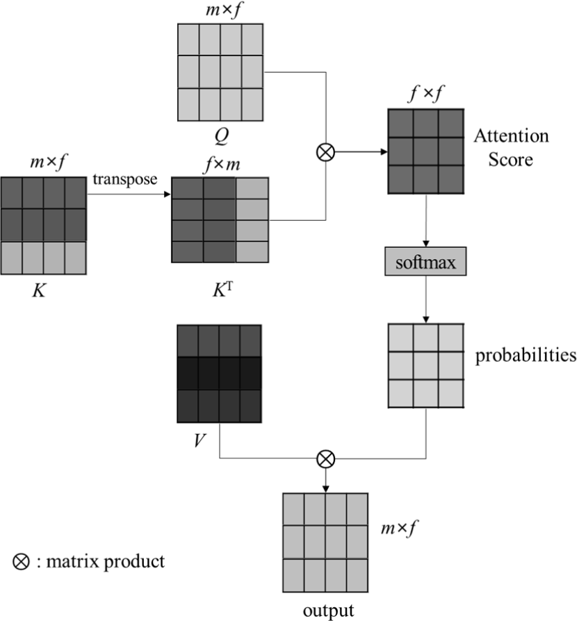
The inputs are required to be converted in order to correctly find the correlations. The m×f attention input can be converted through matrix multiplication with f×f sized learnable tables as shown in Fig. 6. A dot product is performed between each row of the input and each column of the table, then the input is converted to better represent the correlation. It is similar to embedding each word in NLP. The three inputs are converted through referring the tables as follows:
where XQ, XK, and XV are the query, key, and value, respectively, and ⊗ is a matrix product operator. An attention score, which is a correlation between the query and the key, is calculated through dot products of Q and K as follows:
The matrix product between Q and transposed K is equal to the dot products between rows of Q and K. The matrix product result is divided into f in order to make the attention score less affected by the feature length. The attention score can be converted as probabilities for elements through softmax function. The weighted sums of the value are calculated through the probabilities as follows:
Fig. 7 illustrates the flow of attention though equations (3)–(4). A feed-forward neural network (FFNN) makes the attention results non-linear. The FFNN consists of two fully-connected layers as follows:
where α1, α2, β1, β2 are learnable matrices, ⊙ is an element-wise product operator, and σ(·) is an activation function. In the proposed method, the activation function is a parametric rectified linear unit (PReLU). The output of PReLU is equal to its input if the input is positive, otherwise it is the input multiplied by a learnable variable a as follows:
XQ is added to the result of equation (5), that is a residual block. It leads an output close to 0. Then, layer normalization is applied. The residual block and layer normalization improve a network training. We express the series processes in the attention module in equations (2)–(5) as attn. (XQ, XK, XV).
For the target block, self-attention is applied n times to predict the correlation between pixels in the target block. The multiple attentions obtain both the global and local correlations of the input block. A following equation represents the pth result of self-attention:
where is the pth result of self-attention. The correlations between the pixels of the target block and the reference pixels are predicted as follows:
where A is a m2×f correlation map between the target block and the reference pixels and Sref is a 2m×f map which is concatenated between SV and SH as follows:
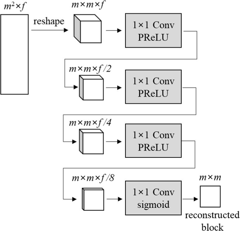
The first dimension of A is divided into two dimensions m×m. Then, the feature dimension is reduced through four CNN layers with 1×1 kernel size. PReLU is utilized as activation functions for the layers except the last. The activation function of the last layer is Sigmoid whose output is between 0 and 1. Fig. 8 shows the structure of the layers for the pixel reconstruction.
For training the proposed network, several videos are utilized. Frames in each video with a gap of 20 are divided into 2m×2m blocks. Each block is included in the dataset for the network training if it satisfies a following conditions:
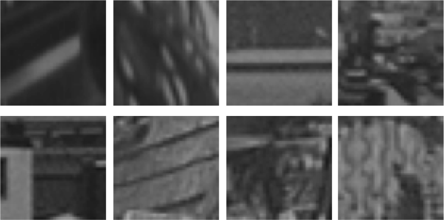
where Btop, Bleft, and Btarget are the top, left, and target blocks, respectively, max(·) and min(·) are the maximum and minimum pixel values of the block, respectively, and t is a threshold. Equation (10) means that blocks whose pixels have similar colors are excluded from the dataset in order to increase learning efficiencies. Fig. 9 shows the samples of the block for the network training. For a total of 120,000 blocks in the dataset, the 100,000 blocks are utilized to train the proposed network and the others are to verify it. A loss function for the network training is a mean square error (MSE) between the target block and the reconstructed block.
IV. SIMULATION RESULTS
For the comparisons of the reconstruction accuracies by the network parameters m, f, and n, we measure reconstruction MSEs for the validation set in the dataset. The default m, f, and n are 16, 24, and 6, respectively. t in equation (10) is specified as 50. The hyper parameters for the network training are as follows: the number of a batch size, the number of epochs, and a learning rate are 128, 300, and 1×10⁻³, respectively.
Table 1 shows the reconstruction MSEs by the number of self-attention times n. The errors of the block reconstruction tend to reduce as n increases. The optimal n is 6 with an MSE of 254.33. When n is 8, the network performance is rather worse. If n overly increases, it leads to overfit during network training due to excessive complexity.
| n | 1 | 2 | 4 | 6 | 8 |
|---|---|---|---|---|---|
| MSE | 364.28 | 270.28 | 259.38 | 254.33 | 257.80 |
Table 2 describes the MSEs by the number of the spatial features f. The reconstruction accuracy of the proposed network increases as the spatial features are more. However, the accuracy increase rate is reduced if f is greater than 24. Although the reconstruction accuracy is better for larger f, the network complexity also increases.
| f | 8 | 16 | 24 | 32 |
|---|---|---|---|---|
| MSE | 274.79 | 270.32 | 254.33 | 254.18 |
Table 3 shows the MSEs by the target block size m. The block reconstruction is harder as the block size is larger. It is more difficult to find the spatial correlations between the reference pixel and the target block as the block size larger.
| m | 16 | 32 | 64 |
|---|---|---|---|
| MSE | 254.33 | 391.96 | 541.13 |
We evaluate the proposed network by comparing prediction results through the intra modes of video coding standard. The intra modes reconstruct a block using adjacent top and left pixels, similar to the proposed method. Several video coding standards such as AVC, HEVC, and VVC provide various intra modes. The intra modes of VVC, which is a state-of-the-art video coding standard, is chosen for the performance comparison with the proposed method. The intra modes are classified into following the type of referring to adjacent pixels: DC mode, planar mode, and angular mode. DC mode reconstructs the block as the average of the reference pixels. In planar mode, the pixel value of the block is calculated through a linear interpolation in horizontal and vertical directions. Angular mode reconstructs each pixel in the block with the reference pixels located at a specified angle by a mode index. VVC has 67 intra modes including a DC mode, a planar mode, and 65 angular modes. VVC selects the best reconstruction results of its intra modes.
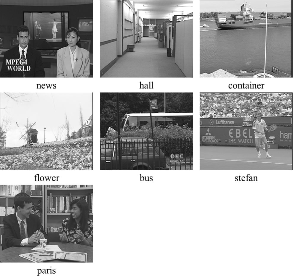
We measure the accuracies of the proposed network for the first frames of 7 actual videos as shown in Fig. 10. The frame is divided into several 32×32 blocks. For each block, MSEs are calculated by selecting best methods among the VVC intra modes and the proposed method. Table 4 shows the comparisons of the MSEs with reconstructing by only the VVC intra modes. The proposed network reduces the average MSE by about 14.8%. The proposed method more accurately reconstructs the blocks than VVC intra modes for at least 27% of the blocks.
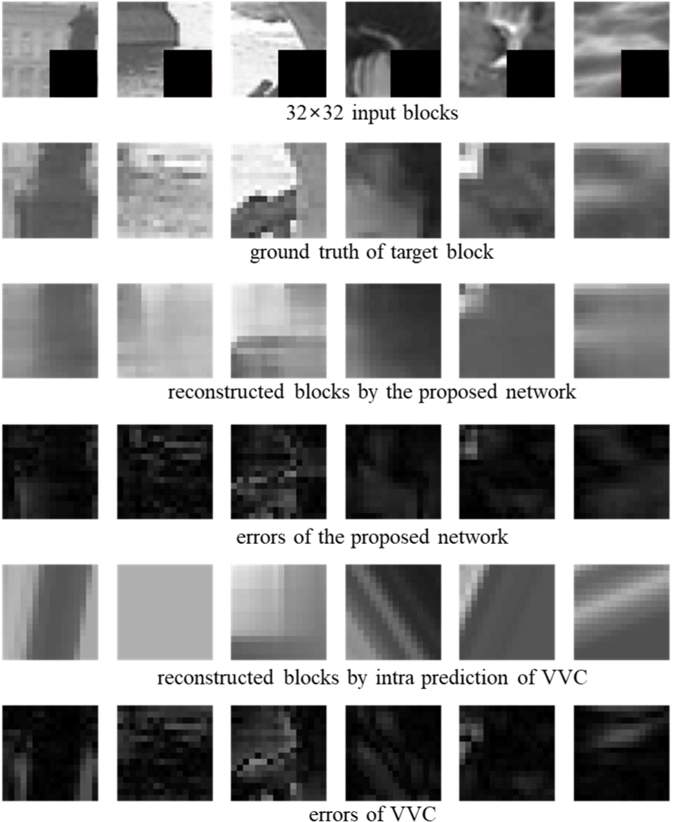
Fig. 11 shows reconstruction results by the proposed network. In Fig. 11, the first row is 32×32 input blocks which are masked for 16×16 target blocks, the second row is ground truths, that are target blocks, the third and fifth are the reconstruction results by the proposed method and by VVC intra modes, respectively, and the fourth and sixth rows are the errors between the reconstruction results and the ground truth. The proposed network further improves the accuracy of the reconstruction for the blocks including more nonlinear patterns such as curves. VVC intra modes can predict pixels only in a single direction, but the proposed method reconstructs the target block by referring to the pixels with high correlation for each pixel.
V. CONCLUSION
In this paper, we proposed the block reconstruction method by predicting the spatial features of the target block. The spatial features were extracted from the pixels of the top and left adjacent blocks through the CNN layers. The spatial correlations between the target block and the reference pixels were predicted by attention mechanism. The pixels of the target block were reconstructed through the CNN layers. In the simulation results, the average accuracy of the reconstruction was 14.8% for the actual videos. In the future, we will continue to conduct research on applying the proposed method to intra-picture prediction for video coding. The proposed network can be applied to video coding, inpainting, and super-resolution.

